CO2 transfer across the air-water interface

The question

The exchange of CO₂ between the atmosphere and lakes, rivers and the ocean is part of the global carbon cycle, and it feeds into climate models and estimates of ocean carbon uptake. Natural and polluted waters carry dissolved salt and surfactants. Salt changes the water's transport properties and how much CO₂ it can hold. Surfactants collect at the surface as a film that can get in the way of the exchange.

Most of the resistance to CO₂ transfer sits in a thin layer of water just below the surface, where CO₂ moves only by molecular diffusion. My dissertation measures how salt and surfactant change the rate across that layer.

The stagnant-film model

The stagnant-film model treats the air above the interface and the water below a thin film as well mixed. Inside the film, of thickness L, CO₂ moves by diffusion alone. The flux per unit area is set by a transfer velocity k_L:

F = k_L (C_surf − C_bulk), k_L = D / L (laminar)

C_surf is the dissolved CO₂ concentration at the interface and C_bulk the concentration in the water below. Turbulence thins the film and raises k_L. Beyond the laminar case, k_L has to be measured, because it depends on turbulence, surfactants, bubbles, temperature, and the properties of the gas and water.

Fig. 1. The stagnant-film picture. CO₂ concentration is uniform in the well-mixed air and water and falls linearly across the film, where transport is by diffusion alone.

Experimental setup

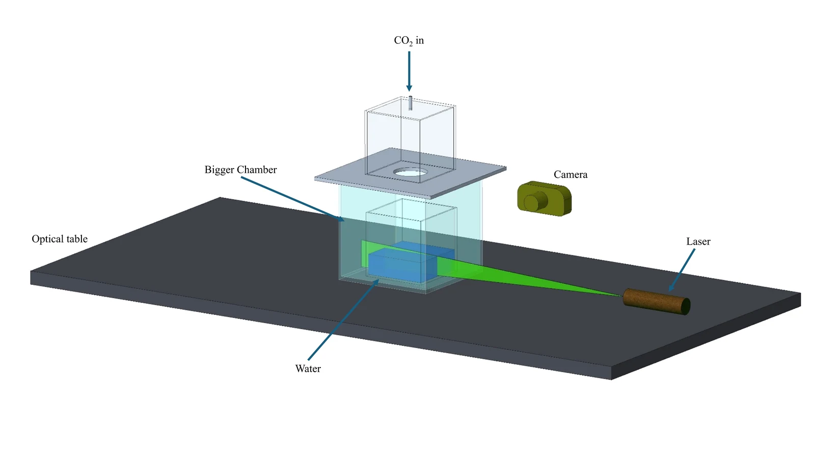
I use two setups. The first shows how CO₂ dissolves. A 10 cm water tank sits inside a larger sealed chamber, with CO₂ fed in from the top. The water carries uranine dye at 1.0 × 10⁻⁵ mol/L, a 532 nm laser sheet makes it fluoresce, and a Nikon V1 camera records the sheet from the side. Dissolved CO₂ lowers the pH, which dims the dye, so CO₂-rich water shows up dark. This planar laser-induced fluorescence (PLIF) is qualitative. It shows where the CO₂ goes but cannot give a transfer velocity.

3-D rendering of the PLIF setup on an optical table: a small water tank inside a larger chamber with a CO2 inlet on top, a laser projecting a green sheet into the tank, and a camera beside it. — **Fig. 2.** The PLIF setup. The water tank sits inside a larger chamber, with CO₂ fed in from the top, the laser sheet entering from the side, and the camera at right angles to the sheet.

The second setup measures the transfer velocity. A 15 cm tank, half filled with water, is sealed with a known amount of CO₂ in the air above it, at a partial pressure of no more than 1.5 kPa. A Vernier Go Direct CO₂ sensor tracks the CO₂ concentration in that air. A Corning magnetic stirrer turns a 2.5 cm magnet at 200 rpm in the water. Salt concentration ranges from 0 to 35 g/kg.

ProgramMore than 500 experiments on CO₂, O₂ and air transfer into water, in sealed chambers of 3 to 4.5 L
SolutesSalt up to 35 g/kg, sucrose up to 200 g/kg, surfactant up to 100 mg/kg
MixingMagnetic stirrer in the water up to about 1,000 rpm; a fan in the air at five settings
Result rangeTransfer velocities from 0.5 to 20 cm/h

The measurement is sensitive to the room. Temperature changes the solubility of CO₂, and humidity controls evaporation, which cools the surface and can drive a flow of its own. Each run starts with a stabilization dwell that holds the temperature within ±0.1 °C and the relative humidity at 95%.

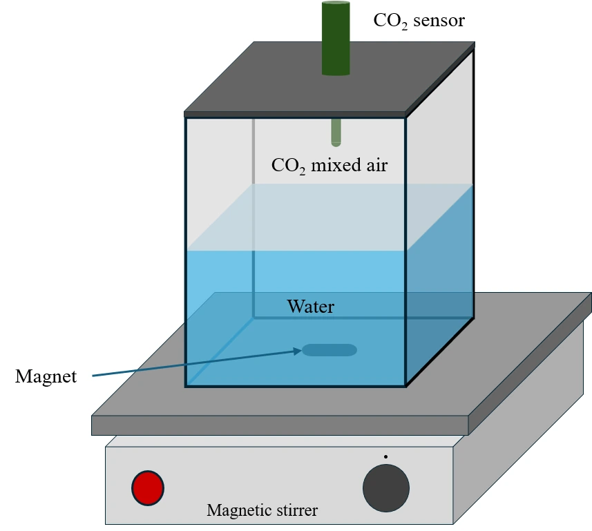
Schematic of the transfer-velocity setup: a closed transparent tank on a magnetic stirrer, water in its lower half with a magnet at the bottom, CO2-mixed air above, and a CO2 sensor reaching through the lid into the air. — **Fig. 3.** The transfer-velocity setup. The sealed tank holds water below CO₂-mixed air. The sensor in the lid tracks the CO₂ in the air while the magnetic stirrer mixes the water.

Because the chamber is sealed, every mole of CO₂ that leaves the air enters the water. With air volume V_a, water volume V_w, interface area A and dimensionless solubility α, the CO₂ concentration in the air c_a decays toward its equilibrium value c_∞ = N / (αV_w + V_a), where N is the total CO₂ in the chamber. Integrating that decay between two times gives

k_L = V_aV_wA(αV_w + V_a)(t₂ − t₁) ln c_a1 − c_∞c_a2 − c_∞

So the transfer velocity follows from the CO₂ concentration in the air alone, measured over time.

Seeing CO₂ dissolve

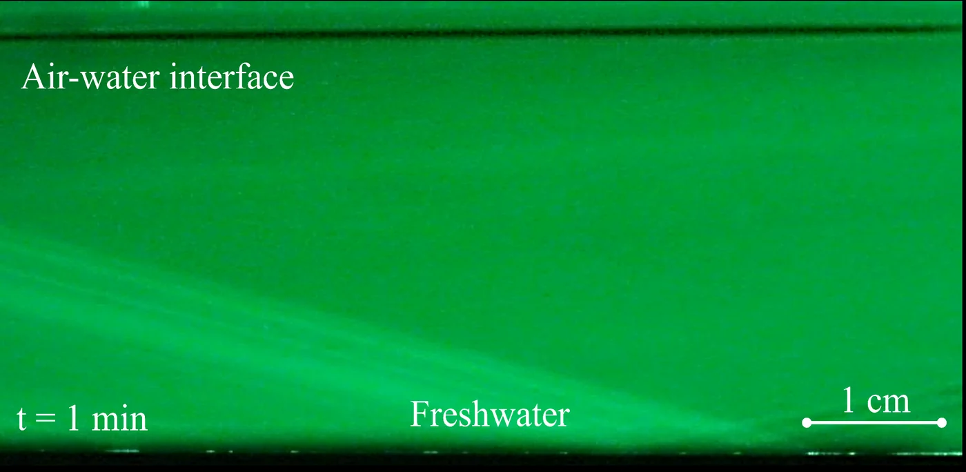
In fresh water, one minute after CO₂ enters the air, the water is still evenly bright and the CO₂ has only reached a thin layer at the interface. Ten minutes later, dark CO₂-rich water has spread well below the surface.

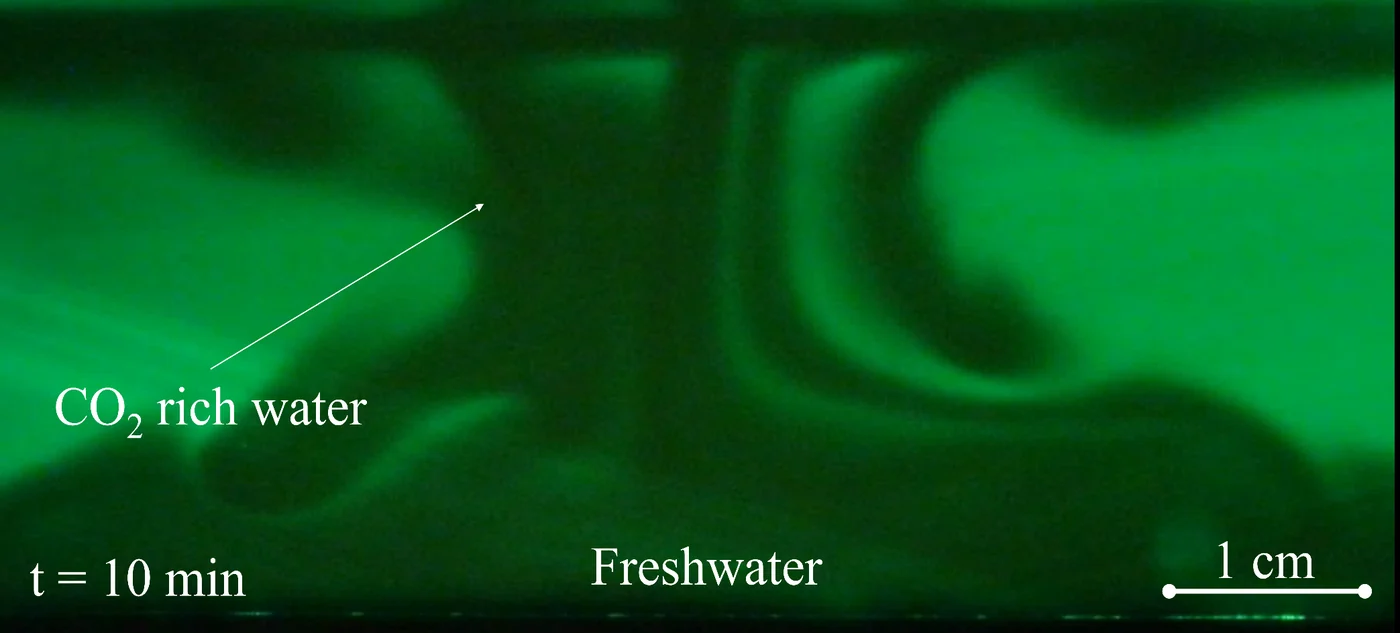
Green PLIF image of fresh water one minute after CO2 was introduced: evenly bright water below a dark line at the air-water interface. Scale bar 1 cm. — **Fig. 4.** PLIF images of fresh water (a) one minute and (b) ten minutes after CO₂ was introduced into the air above it. Dark regions are rich in dissolved CO₂. Scale bars are 1 cm.

Green PLIF image of fresh water ten minutes after CO2 was introduced: large dark regions of CO2-rich water swirl well below the surface. Scale bar 1 cm. — **Fig. 4.** PLIF images of fresh water (a) one minute and (b) ten minutes after CO₂ was introduced into the air above it. Dark regions are rich in dissolved CO₂. Scale bars are 1 cm.

Recorded over a longer time, a plume of CO₂-rich water sinks from the surface with a strong downward flow and reaches the bottom of the tank.

Video 1. PLIF recording in fresh water, starting ten minutes after CO₂ was added above the water. The first two minutes are shown, played ten times faster. The bright line at the top is the air–water interface, and the specks are tracer particles.

Transfer velocities

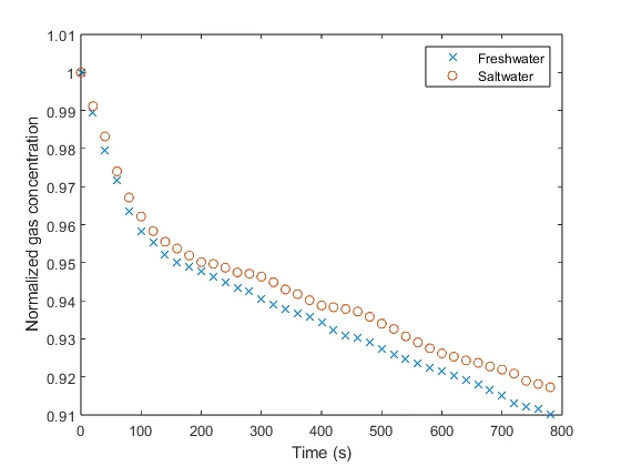
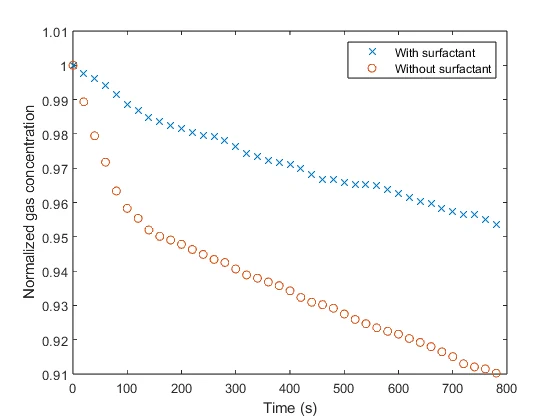
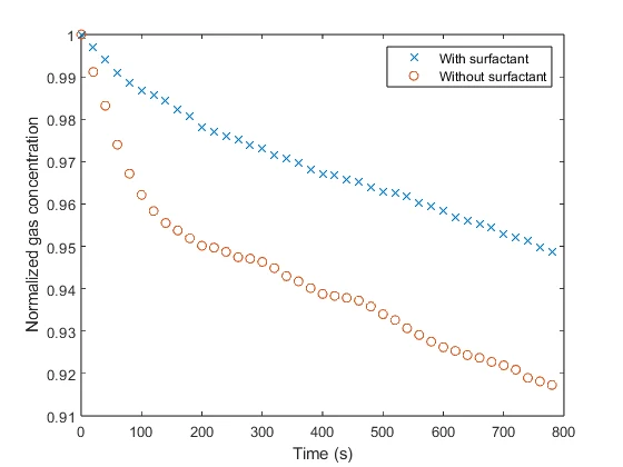
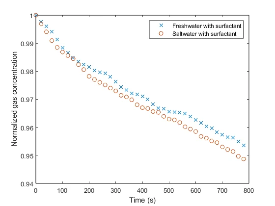
Each run starts with a fixed amount of CO₂ in the air and follows its concentration as the water absorbs it. The runs started at slightly different amounts, so each curve is normalized by its starting value. A faster drop means faster transfer into the water. These runs used the stirrer at 200 rpm.

Normalized CO2 concentration in the air against time for fresh water and saltwater; both fall from 1.0 to about 0.91 over 800 seconds, fresh water slightly faster. — **Fig. 5.** Normalized CO₂ concentration in the air over 800 s for (a) fresh water vs saltwater, (b) fresh water with and without surfactant, (c) saltwater with and without surfactant, and (d) fresh water vs saltwater, both with surfactant. Panels read left to right, top to bottom.

Normalized CO2 concentration against time for fresh water with and without surfactant; without surfactant it falls to about 0.91, with surfactant only to about 0.95. — **Fig. 5.** Normalized CO₂ concentration in the air over 800 s for (a) fresh water vs saltwater, (b) fresh water with and without surfactant, (c) saltwater with and without surfactant, and (d) fresh water vs saltwater, both with surfactant. Panels read left to right, top to bottom.

Fig. 6. Measured CO₂ transfer velocity for the four waterbodies, at a stirrer speed of 200 rpm.

Salt
The transfer velocity drops from 7.2 cm/h in fresh water to 6.1 cm/h in saltwater, about 15% lower. Salt lowers both the solubility and the diffusivity of CO₂ in water, which may explain the drop.
Surfactant
Surfactant roughly halves the transfer velocity, to 3.4 cm/h in fresh water. This is consistent with a surfactant film at the interface acting as a barrier.
Both
Saltwater with surfactant has the lowest transfer velocity, 3.2 cm/h, slightly below fresh water with surfactant.

Surfactants from pollution could therefore slow how fast natural waters take up CO₂, with consequences for the carbon cycle.

Modeling the uptake

Alongside the experiments I built a 2-D simulation in MATLAB of CO₂ dissolving into still water beneath a closed headspace. Dissolved CO₂ makes water slightly denser, by only about 0.02 kg/m³ at saturation here. That is enough. The CO₂-rich layer at the surface grows heavier until it breaks into finger-like plumes that sink and carry CO₂ down far faster than diffusion can. The model shows the same kind of sinking plume that the PLIF video records in fresh water.

The model couples the incompressible Navier–Stokes equations, with the Boussinesq approximation for buoyancy, to CO₂ advection and diffusion in the water. A well-mixed mole balance tracks the headspace, and Henry's law links the two at the interface, so the gas side depletes as the water absorbs. A diffusion-only run, identical in every other way, is the reference.

DomainVertical slice of the tank, 10 cm wide and 2 cm deep
Gas sideClosed 0.8 L headspace, CO₂ at 6 kPa initially
Grid360 × 180 staggered (MAC) cells, adaptive time step
NumericsIncremental pressure-correction projection, van Leer TVD transport
RayleighRa ≈ 8.5 × 10⁵ at the start
ChecksMatches the analytical erfc solution to within 0.01%; CO₂ conserved to round-off

Video 2. Thirty minutes of simulated CO₂ uptake. Top, with density-driven convection; bottom, diffusion only. Color shows the dissolved CO₂ concentration, with the air–water interface along the top edge. Frames come from a rerun of the same script that saves the field every 10 s.

Onset
For the first 12 minutes, CO₂ enters by diffusion alone and the two runs are indistinguishable. At about 12.5 minutes the surface layer goes unstable and the transfer velocity climbs above the diffusion-only value.
Peak
Once the plumes form, the transfer velocity reaches up to 4.2 times the diffusion-only value.
After 30 min
The water holds 1.7 times as much CO₂ as it would by diffusion alone.

Fig. 7. Total CO₂ dissolved in the 0.2 L of water, with and without density-driven convection. From the MATLAB results of the two runs.

Status

The manuscript, Gas transfer across the air–water interface and its dependence on dissolved solutes, is in preparation. I presented the work at the 2024 APS Division of Fluid Dynamics meeting and at the APS March Meeting 2026, with K. Jawney, I. Benouaguef, I. S. Fischer and P. Singh.

This work builds on our study of Marangoni flow induced by a raindrop, where the same salt and surfactant effects set the direction of the surface flow.